We all know that the game of beer pong is relatively simple in terms of physics. What this post presupposes is: maybe it isn't?

Before I even begin, I'd like to say that if you are looking for pretty pictures and advice, skip to Optimal aiming or Beerpong fractals. Otherwise, enjoy.

First, I feel like I have to explain what the game beer pong is. And let me tell you, it is exactly what it sounds like - a small white ball bouncing between two paddles on an Atari while two gentlemen sip beverages. Well, fine, it's dudes throwing balls into cups full of beer until their girlfriends leave for another party.

Now, what are typical questions that one may ask when thinking, "hmmm, I'm bored and want to know about the physics of beer pong"? They may include:

1. What is the precise trajectory I need to make it in a cup?
2. Where should I aim, given my ability level?
3. If I shot randomly at the cups what is the chance that I make it in?

I will sort of touch on these issues, but only through a completely different question - what happens when we don't quite make it? What happens when the ball bounces off the rim? Now there's something to make your socks go up and down.

Creating trajectories

Okay, so everyone who has encountered physics knows that we can describe a ball flying through air with a quadratic equation (except maybe Michael 'Air' Jordan who simply has no regard for gravity). It looks something like this:

$$ y(t) = y_0 + v_{0,y}t - \frac{1}{2}g t^2 $$ $$ x(t) = x_0 + v_{0,x}t $$ $$ z(t) = z_0 + v_{0,z}t $$

where y is up, gravity is down and there is no air resistance. I feel like I have to bring up this point unncessarily early. I do physics, not real things. Air resistance would make this real. Real hard. So it's gone, like my hopes of growing up to be an astronaut. So, when you throw a ball, you can determine at any time where it is, where it's going and which dreams it's left behind along the way. This is going to be useful to us later, so don't forget it.

Alright, so I guess we need to make some cups and balls and and then throw them at one another. Let's do it.

A cup rim is a torus. A ball is a sphere. Bill Murray is my hero. These are just facts. What is a little more contentious is that for the rest of this post, I want to simplify the interaction of the cup rim and ball to a single torus, leaving the ball to be an infinitessimal speck. Imagine attaching one of those awesome spherical neodymium magnets to a metal hoop and swinging it around until the ball rolls over the entire surface. The center of that sphere would trace out the surface of a torus. I hope that's convincing since I'm not going to try again. I tried to make a picture but it didn't turn out great.

Finding collisions between this infinitessimal ball and ball-rim torus amounts to finding the intersection of the equation of torus and that of a parabola. This is because we ignored air resistance; if we didn't, it would be some other minimization algorithm which wouldn't be too terrible, but probably not fun either. In terms of polynomials, a torus can be written

$$ (x_n^2 + y_n^2 + z_n^2 + R^2 - r^2)^2 = 4R^2(x_n^2 + y_n^2) $$

where $x_n$, $y_n$, $z_n$ are normalized coordinates, $x_n = x(t) - x_c$ where $x_c$ is the center of the rim. And all the rest are normalized too. We can then plug our previous equations, setting $x = x(t)$ where $x(t)$ is the coordinate from earlier, and get an 8th order polynomial in time. You can convince yourself it's 8th order just by starring at the equation or realizing how many times a cricket wicket could intersect a jelly doughnut. Well, actually, just a regular doughnut since we need the hole gone.

Okay, now that we know every time (literally, the variable is $t$) the ball intersects the rim, we have to figure out what happens when it bounces off. It's just like bouncing on a table, except that table is a torus and so only flat in a small region. So, we find the normal of the rim at the collision point, and reflect the ball about this normal. Easy, breezy, toroidal cover girl.

For a quick recap (for science and reproducability and all that...):

1. Give initial trajectory to a single infinitessimal ball
2. Find all 8N possible collisions with a torus (technical: Bairstow's method) , where N is the total number of cups that it could possibly collide with
3. Determine the closest collision in time, throwing away those in the past
4. Move to that collision point
5. Determine the normal vector on that part of the torus and reflect the current velocity.
6. Start again, and continue until the next collision time never occurs or it occurs after the ball crosses the zero plane.

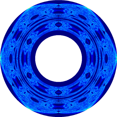
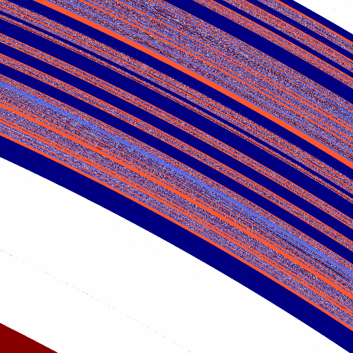
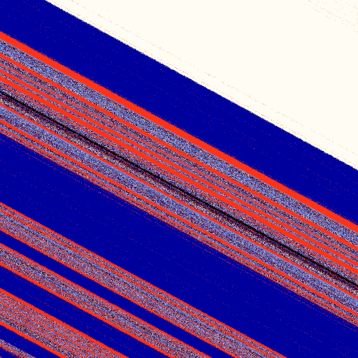
Finally, we can start to look at some pictures a.k.a. was that a bunch of nonsense or is there a reason that this post goes on for 3 more pages. Let's drop ten thousand ping pong balls from straight above a single cup rim and look at the surface of interaction where they touch. It looks like this:

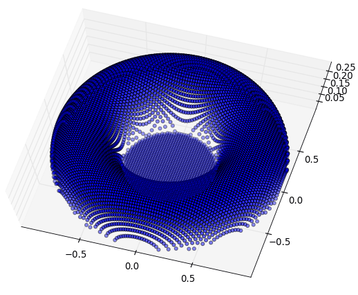
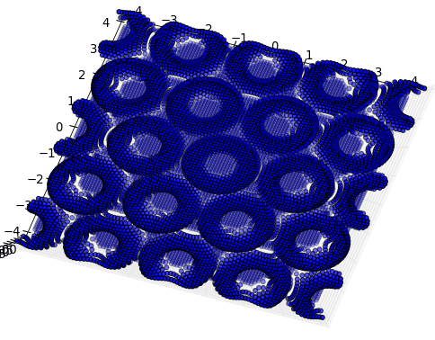
The second picture is for an infinite array of cups, which we will be looking at in the fractals and scattering sections. Looks like we're doing okay so far. Okay, okay. It's actually a little more subtle - there are a lot of parameters that we need to start thinking about. Next we'll describe them and look at various configurations of these torii.

Physical setup

Now I'm going to put on my 'physics in the real world hat' and put some numbers behind all these letters. Our variables are: $R$ is the radius of the cup, $r$ is the radius of the ball-rim, $h$ the height of the drop, $\eta$ fractional restitution coefficient ($v_{n+1} / v_n$ between bounces), and... I think that's it. Except $x_0$ and $v_0$. And $\epsilon$, the cutoff resolution of root finding. Oh, and $g$, the gravitational constant. I was close.

To simplify our numbers, I will be presenting non-dimensional forms of these variables, normalized by the inter-cup spacing $D$, from center to center. On a serious note this is a very important technique in physics and can give you great insight into the importance of different physical processes in a situation. However, the choice of this normalization may not have been the best as it is used mainly for historical reasons, for which you can blame the author. Using a standard solo cup, we find that

$$ R/D \approx 0.95, \,\,\, r/D \approx 0.30, \,\,\, \eta \approx 0.3, \,\,\, \frac{g D} {|v_0|^2} \approx 1, \,\,\, \epsilon \approx 10^{-15} $$

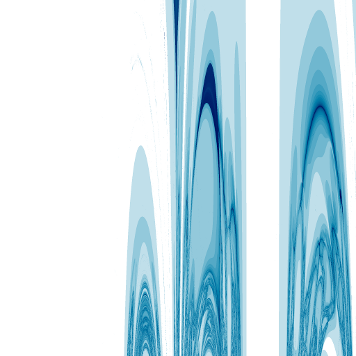
Let's start again with a quarter million balls dropped directly overhead a cup from a height $h \approx 6\,\rm{ft}$, $h/D \approx 20$ and color the pixel of where it started according to how many times the ball bounced before it went into a cup (darker is fewer). And let's start with the infinite array of cups for curiosity's sake. When we do this, we see a very cool pattern. Of course we can see the center of the cup where there are no collisions. The hexagonal symmetry also appears, as well as 'images' of the other cups on the rim of the center cup.

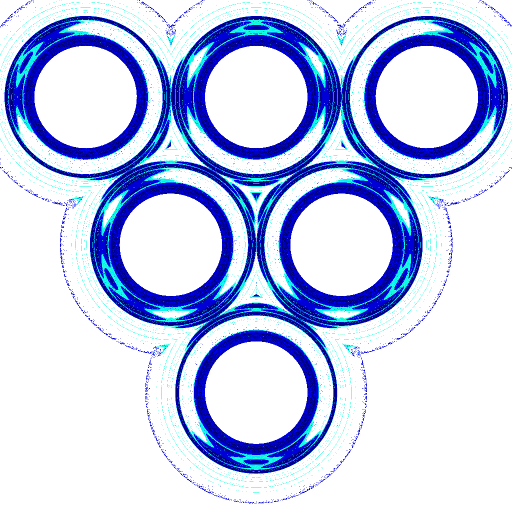
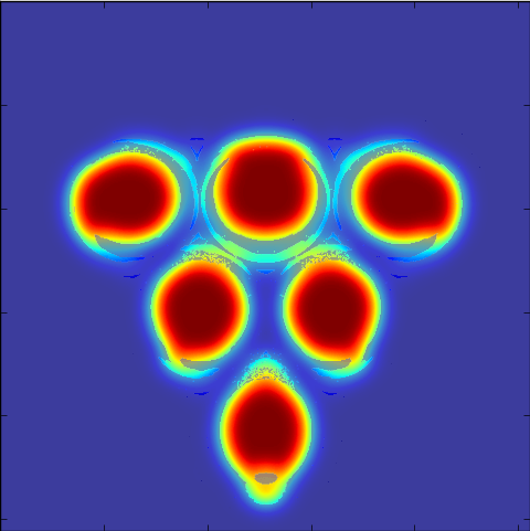
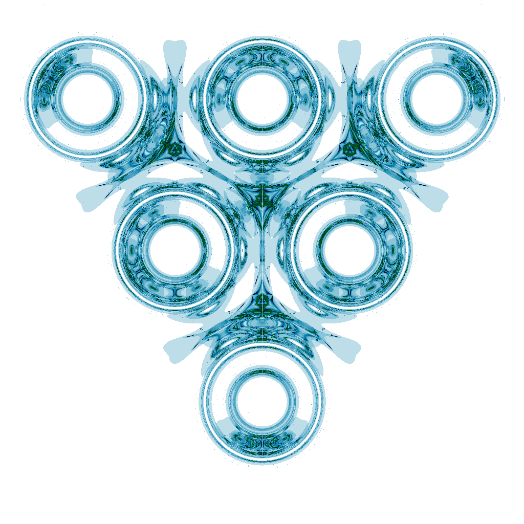
But, who actually has an infinite number of solo cups laying around? Let's go for the physically reasonable 6 cups and color only the throws that actually end up in a cup by the time they're done bouncing. We still see the requisite symmetry and we can start to see where some of the bounces map. On the back row, the darker colors represent nearest neighbor bounces while the lighter color is a double bounce from second nearest neighbor to another another cup.

Optimal aiming

Until now, we've been investigating how to properly simulate beerpong and getting a feel for the parameter space. Let's answer some so-called 'real' questions now. For example, where should you aim?

To answer this question, we'll tilt our previous 6 cup simulation so that the launch position is at eye level from 6 ft. away. From there, let's make our usual bounce count picture, but now in $\theta-\phi$ space, the angles associated with the throw. Doing so, we can see the bias between front and back of the formation, with the effect of the back row being a backboard ('KOBE!').

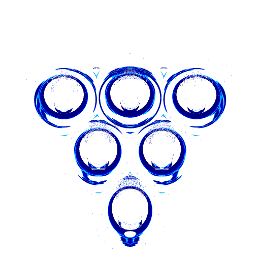
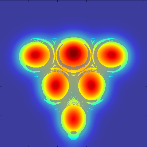
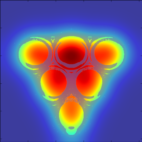
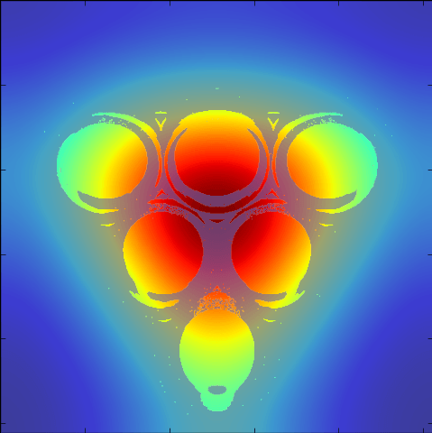
But of course, people can't aim perfectly (except Michael 'Laser Fingers' Jordan who doesn't know the meaning of uncertainty) so let's start to blur our eyes. We blur the pattern of shots that land in a cup by various levels of gaussian kernels. The size of the variance approximately models various levels of aiming ability. Looking at these various errors levels in fractions of the cup size, we see

• 10% - you're pretty talented. Have too much free time? In either case, just aim for the center of the cup, you can do it, I believe in you.
• 33% - aiming towards the center of the center back cup actually starts to help.
• 50% - you're teammates, friends, associates, and puppy will like you better if you aim for that back center cup. That is of course ignoring the fact that this is bad overall strategy, but that's not the question we are addressing.
• 100% - you can't hit a cup. You should just aim for the center of the entire setup. It works out better for you that way.

Beerpong fractals

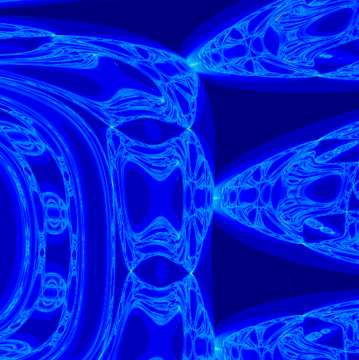
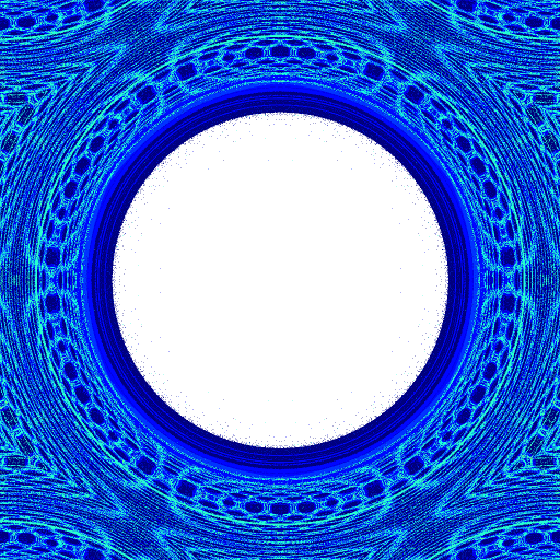
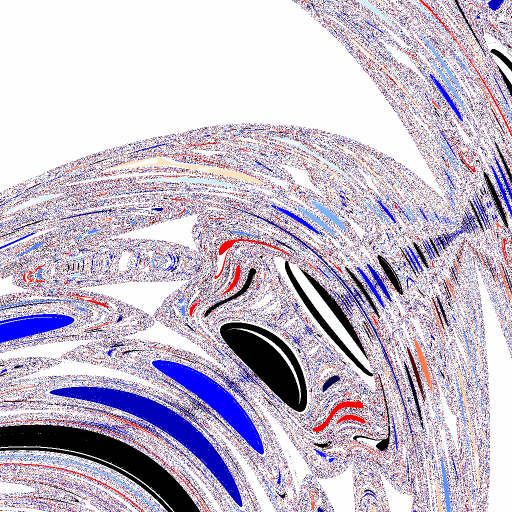
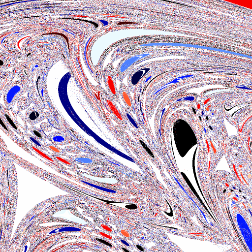
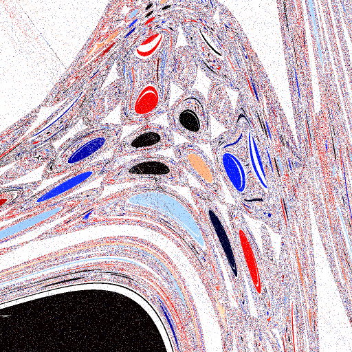
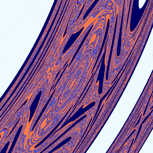
Alright, that was way too applicable, we gotta bring it back. So, finally, as I promised, let's investigate those weird cup images that we saw in the infinite lattice pictures. Let's back up from the realm of physically viable parameters. I'm talking thin cups that have some infinitessimal separation between them and a ball so bouncy that it could be marketed as magic. Our parameters are

$$ R/D = 0.7, \,\,\, r/D = 0.30, \,\,\, \eta = 0.9 $$

Let's drop balls from directly overhead from a significantly lower height (for numerical accuracy reasons). On the edges we see where the ball can just barely fit between the cups while bouncing around violently. I'll call these elbows. Why? I'm not really sure. But soon, we will see elbows all the way down. Let's choose an interesting area and zoom way, way in. I mean, given the scale of the cup, let's go atomic scale, $1\, \overset{\circ}{\rm{A}}$. We can see that the elbow features occur everywhere. In fact, many different features occur until the very smallest scales - a fractal.

Below is a little javascript program that allows you to zoom through the many levels of the beerpong fractal. After you click load and allow the images to buffer, use the slider to zoom from cup scale to atomic scale and in between.

If we vary the height of the starting position, we can look at the folding and evolution of these self similar structures. Another slider program for this is below:

It is also (arguably) interesting to look at different slices of these same pictures. Let's plot a single $45^{\circ}$ line from the center of a cup to the outer edge along the horizontal axis. In the vertical direction, we can vary the value of the restoration factor, $\eta$. I changed the colormap, but we can still see the elbows that occur and how they appear and spread apart as the restoration coefficient increases.

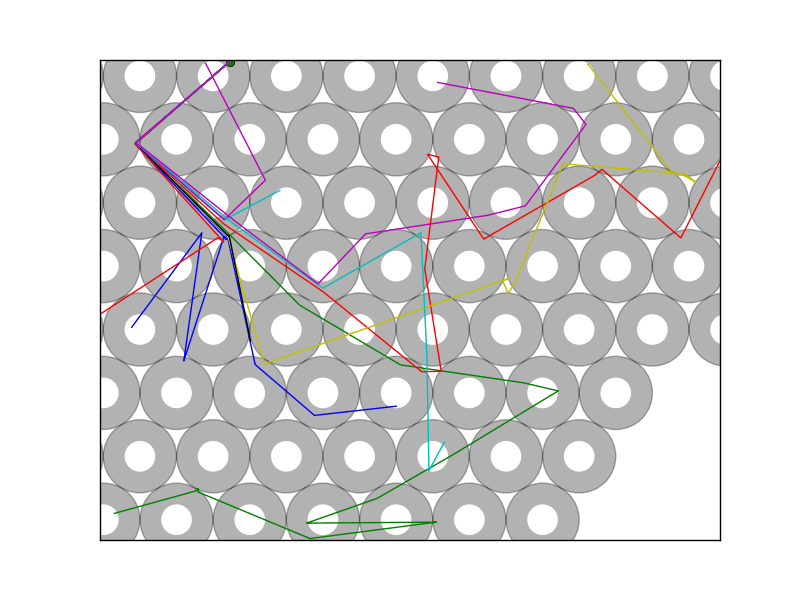
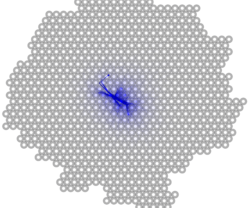
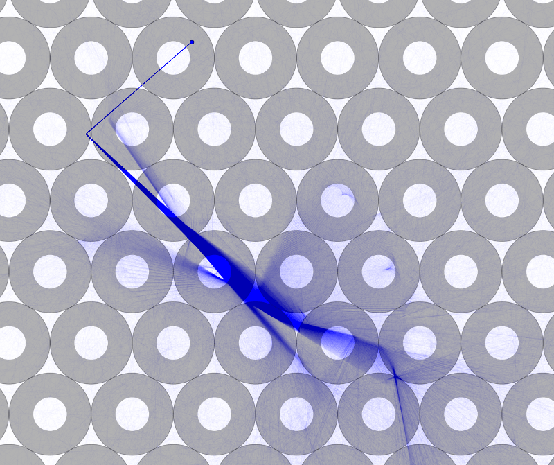
These fractal structures that are shown in the above are really another way of representing an attribute of chaos: sensitivity in initial conditions. That is to say, even the smallest perturbation in a particle's initial trajectory will cause it to quickly diverge away from very similar trajectories. In the beerpong system, we can investigate this property by looking at top down views of pong ball paths. Every kink in the trajectory is a collision with a cup causing it to change directions. We can see that even after just a few collisions, very similar trajectories have moved to entirely different cups.

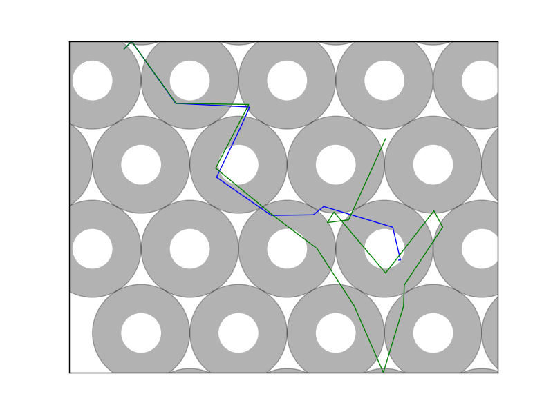
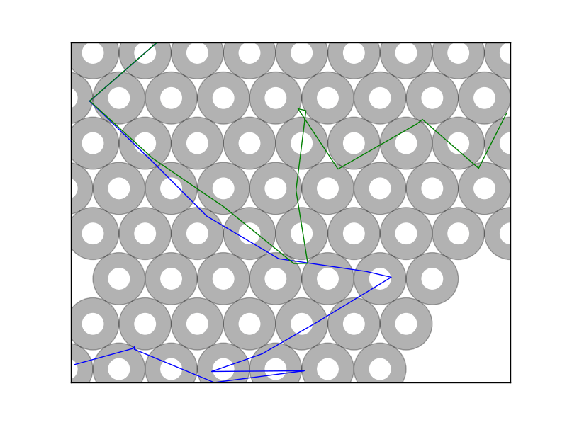
If we sample enough of these paths, you might start to believe that any starting point could potentially reach any other point if you varied the position just right. If you manage to choose your point of interest in one of the boundary regions, it turns out you can do just that. More about that just below.

Chaotic Scattering

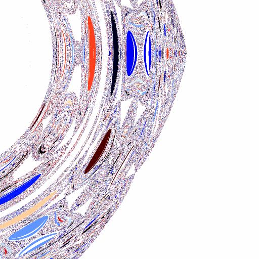
It turns out that the dynamics of beerpong are actually quite closely related to a field in nonlinear dynamics and chaos called chaotic scattering. In these systems, it is common to label trajectories by where they 'exit' the system. In beerpong, this means labeling the old pictures by the cup that the ball eventually ends up in. Doing so, we again arrive at (less pretty) fractals, where we can see the ball going into the same cup on many different scales. In fact by setting the restitution factor to 1, unlike the previous section, we actually see these structures until the point where we run into numerical issues due to floating point limitations. To give you a sense of this scale, if the first scale were the size of the entire earth, the last is the size of a single atom. We could go into 'long double' calculations for a few more bits or use multi-precision, but I don't think there's much to gain.

What's really cool is there is actually a chaotic scattering fractal that you can make and observe in your own home. To do so, stack 4 reflective balls (such as Christmas ornaments) into a pyramid shape, and shine different colored lights through two of the openings and look in one of the other two. Inside, you will see a real-space fractal!

In fact, these are not just any type of fractal, they are 'Wada' fractals in which the boundary between these attractors are fractal. In the case of the shiny balls, each of the colors actually always touches each of the other colors? I'm not sure that made sense. You can read about it more on the wiki.

It appears that beerpong also shares these properties. If we make sure that there is not way for the pong ball to escape without going into a cup, we can start to see these complicated fractal boundaries. Again, these boundaries continue to show more sub-boundaries until our simulation breaks due to rounding errors.

Sources and more

So, remember to shoot towards the center back if you're uncertain and that beerpong is pretty complicated once you don't swish / hole in one / touchdown / I'm bad at sports sayings.

You can find the source code on my github. I also made giant pictures of these beerpong fractals in case you want to make a poster (any one of the pictures below). They are also available for \$60 through email. No, I'm not joking, I'll print one and mail it to you. You're welcome.

Also, I lied about the singularities (its more like non-analyticities but that's not here or there).